---
title: "PART 4 多元线性回归"
---
```{r setup, include=FALSE}
source(here::here("_common.R"))
knitr::opts_chunk$set(echo = TRUE, message = FALSE, warning = FALSE)
```
::: rmdnote
**什么是多元线性回归**
多元线性回归是线性回归的扩展形式,用于分析一个连续因变量与两个或更多自变量之间的线性关系。其模型形式为 Y = a + b1X1 + b2X2 + … + bkXk,可同时考察多个因素对结果的影响。
与一元线性回归相比:一元只含一个自变量,多元含多个;多元能控制混杂变量、评估各因素的独立贡献,而一元易遗漏变量导致偏差;两者均要求线性关系、残差独立正态等前提。
:::
## 10 多元线性回归
作用:用多个影响因素共同预测一个连续结果的变化。
使用范围:因变量必须是连续型。自变量X优先是连续性数值,也可以是二分类。
前提假设(但是和别的不一样,前提假设是放到后面的)
1. 线性关系:每个自变量和因变量之间存在线性关系,自变量之间不存在完美的线性关系;
2. 独立随机抽样:观测值之间相互独立,无自相关
3. 残差正态性:模型残差是Z分布
4. 同方差性:残差的方差不随自变量\\预测值的变化而变化。
5. 无严重多重共线性:自变量之间不能高度线性相关。
### 10.1数据准备与清洗
数据导入:将整理好的数据读入分析工具,要求每一行是 1 个观测样本,每一列是 1 个变量(因变量 Y + 所有自变量 X)
基础清洗:剔除缺失值、重复值,确保变量类型正确(数值型)\
初步异常值筛查:通过散点图、描述统计初步识别极端值,为后续模型诊断做准备。\
*注:这个数据是ai编的,不代表实际情况*
```{r Preparation}
#Preparation


# upload the data导入数据
#library(haven)
x_df<-read_sav(here("data","sav_files","MLR_work.sav"))
attach(x_df)

# str(object) 显示R对象(如数据框)的内部结构,包括变量名、类型和前几个观测值
str(x_df)
head(x_df)
# colSums(is.na(data.frame)) 按列计算缺失值数量,is.na()返回逻辑矩阵,colSums()求和
missing_count <- colSums(is.na(x_df))
print(missing_count)
# 若存在缺失值,可选择删除含缺失值的行(列表删除)
# na.omit(object) 返回删除任何含有NA值的行后的数据框

gender<-as.numeric(gender)
```
或者整理变量矩阵(第一列为因变量Y,后续列为自变量X)\\
这是另一个例子\
m \<- matrix(nrow = length(salary), ncol = 5)\
m\[,1\] \<- salary \# 因变量Y:薪资\
m\[,2\] \<- educ \# 自变量X1:受教育年限\
m\[,3\] \<- salbegin \# 自变量X2:起薪\
m\[,4\] \<- jobtime \# 自变量X3:在职时长\
m\[,5\] \<- prevexp \# 自变量X4:过往工作经验\
然后一定要注意矩阵,矩阵里是只能放数字的。 \
比如有那种二分类的,就把他转成01这样就好 \
有个更快的办法是as.matrix()
\
*别.把.矩.阵.的.英.语.拼.错.了.*
*我。说。怎。么。老。报。错。*
*M.A.T.R.I.X*.
### 10.2 拟合模型前的前置检验
相关性检验:计算所有变量的相关矩阵\
核心目的 1:确认因变量Y和每个自变量X有一定相关性,完全无相关的 X 无需纳入模型; 核心目的 2:初步判断自变量之间的相关性,排查多重共线性风险。
线性关系检验:绘制每个自变量与因变量的散点图,确认二者存在线性趋势,无明显的非线性关系;
样本量校验:对照上述样本量标准,确认样本量满足分析要求。\
*样本量校验就用眼睛看()*
```{r Correaltion-matrix}
#caculate correlation matrix
m<-as.matrix(x_df)
cor_matrix_mlr<-cor(m)
cor_matrix_mlr
# 绘制单个自变量与因变量散点图
#plot(数据框名$自变量名, 数据框名$因变量名,
#main = "自变量X与因变量Y散点图",
#xlab = "自变量X", ylab = "因变量Y")
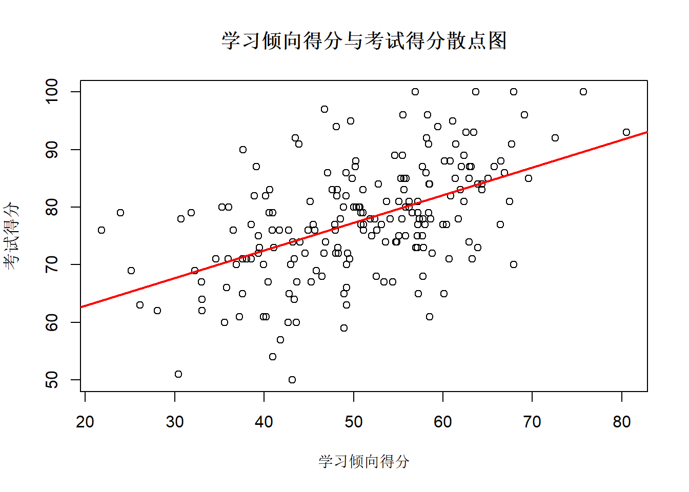
plot(x_df$aptitude, x_df$stats_score,
main = "学习倾向得分与考试得分散点图",
xlab = "学习倾向得分", ylab = "考试得分")
# 添加拟合直线,更清晰看线性趋势
#abline(lm(因变量名 ~ 自变量名, data = 数据框名), col = "red", lwd = 2)
abline(lm(stats_score ~ aptitude, data = x_df), col = "red", lwd = 2)
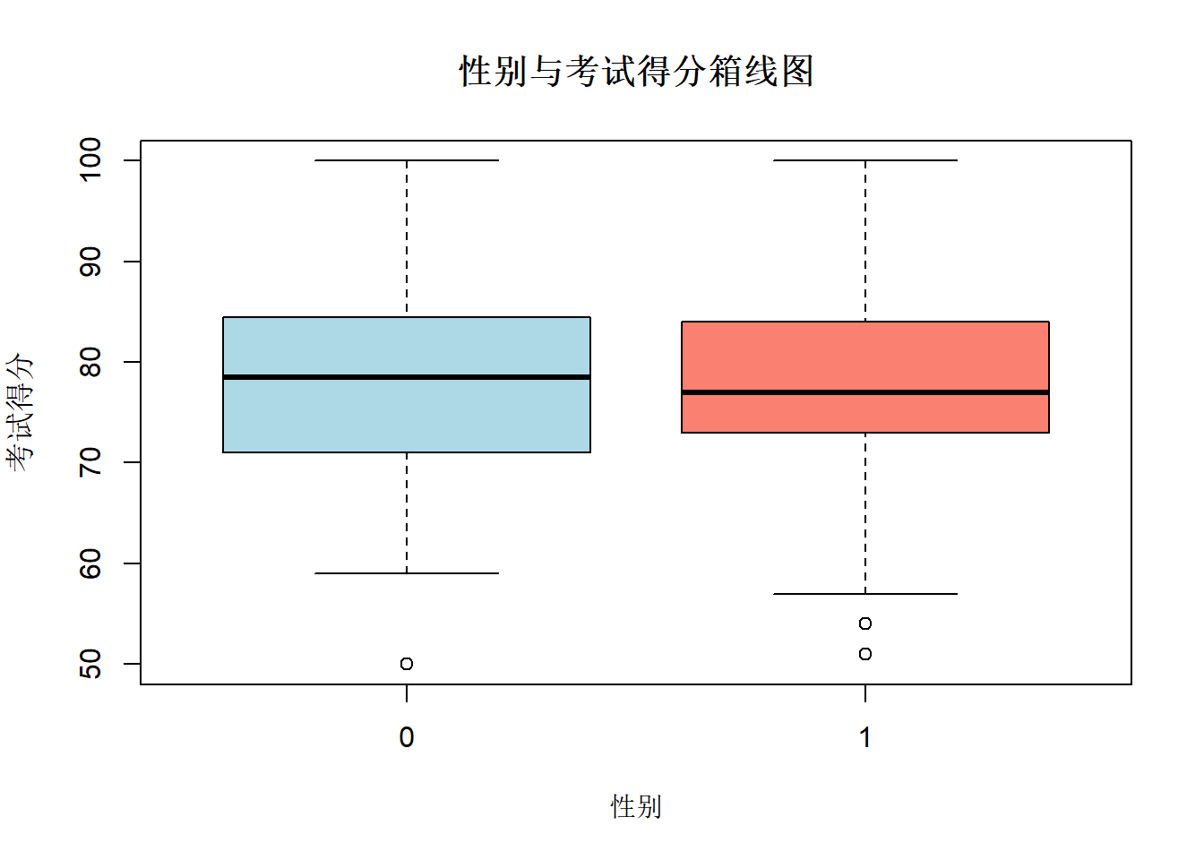
# 绘制 性别 与 考试得分 的箱线图
boxplot(x_df$stats_score ~ x_df$gender,
        main = "性别与考试得分箱线图",
        xlab = "性别",
        ylab = "考试得分",
        col = c("lightblue","salmon"))
# 批量绘制所有自变量与因变量散点图(5列数据用2行3列排版,排的是画出来的小图的板,也就是四个小图放到一个2*3的格子里)
par(mfrow = c(2, 3))
# 循环绘制每个X与Y的散点图(连续性用散点,不连续用箱线)
for (i in 2:ncol(m)) {
# plot(自变量, 因变量)
plot(m[, i], m[, 1],
xlab = colnames(m)[i],
ylab = colnames(m)[1],
main = paste(colnames(m)[i], "vs", colnames(m)[1]))
# 添加线性拟合直线
abline(lm(m[, 1] ~ m[, i]), col = "red", lwd = 2)
}
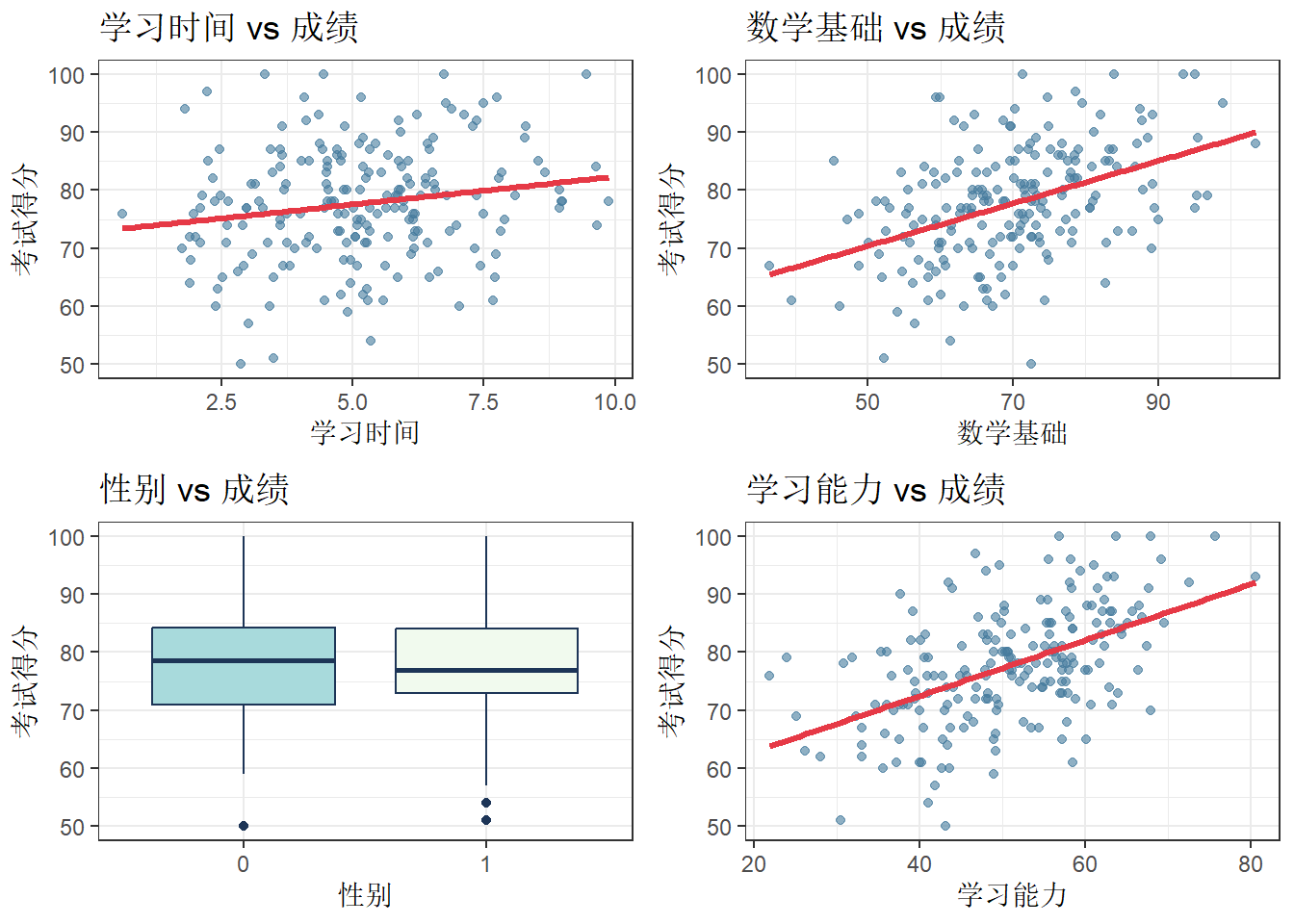
#画出来不是很好看其实。但也凑活。如果想好看点可以参考下面的
df<-data.frame(
学习能力 = x_df$aptitude,
数学基础 = x_df$math_base,
学习时间 = x_df$study_hours,
性别 = as.factor(x_df$gender),#注意,这里有一个很大的区别就是之前的gender是numeric而这个是factor
考试得分 = x_df$stats_score
)
head(df)
# 加载包(如果没装过,先运行一次下面这句)
# install.packages("ggplot2")
#嘴一句,ggplot2真的是万恶之源。
#library(ggplot2)

# --------------- 美观的图(2×2排版)---------------
p1 <- ggplot(df, aes(x=学习时间, y=考试得分)) +
  geom_point(color="#457b9d", alpha=0.6, size=1.5) +
  geom_smooth(method=lm, se=F, color="#e63946", linewidth=1.2) +
  labs(title="学习时间 vs 成绩", x="学习时间", y="考试得分") +
  theme_bw()

p2 <- ggplot(df, aes(x=数学基础, y=考试得分)) +
  geom_point(color="#457b9d", alpha=0.6, size=1.5) +
  geom_smooth(method=lm, se=F, color="#e63946", linewidth=1.2) +
  labs(title="数学基础 vs 成绩", x="数学基础", y="考试得分") +
  theme_bw()

p3 <- ggplot(df, aes(x=factor(性别), y=考试得分)) +
  geom_boxplot(fill=c("#a8dadc","#f1faee"), color="#1d3557") +
  labs(title="性别 vs 成绩", x="性别", y="考试得分") +
  theme_bw()

p4 <- ggplot(df, aes(x=学习能力, y=考试得分)) +
  geom_point(color="#457b9d", alpha=0.6, size=1.5) +
  geom_smooth(method=lm, se=F, color="#e63946", linewidth=1.2) +
  labs(title="学习能力 vs 成绩", x="学习能力", y="考试得分") +
  theme_bw()

# 组合成 2×2 拼图
#library(gridExtra)
grid.arrange(p1, p2, p3, p4, ncol=2, nrow=2)

#其实颜色这一块有个小妙招(井号加一个三位数一般也是一个好看的颜色)
```
### 10.3 拟合多元线性回归模型
核心模型公式:原始分数模型(非标准化): $$Y=α+β_1X_1+β_2X_2+...+β_pX_p+e$$\
α:截距,所有自变量为 0 时 Y 的预测值;
β₁\~βₚ:非标准化回归系数,X 每变化 1 个单位,Y 的变化量\
e:残差,服从均值为 0、方差为 σ² 的正态分布。
\
散点图大家都能看出来,那就讲解箱线图怎么看\
箱体就是中间的长方形,箱体高度代表数据的离散程度:\
箱体越高,数据越分散;越低,数据越集中 下沿 = Q1(第 25 百分位数),\
上沿 = Q3(第 75 百分位数)
\
R²(多重决定系数):模型解释的 Y 的变异 \\ Y 的总变异,取值 0\~1,越接近 1 说明模型解释力越强; 当自变量之间完全不相关时,R²= 每个自变量与 Y 的相关系数的平方和; 当自变量之间相关时,需扣除重叠的方差,R² 小于平方和。
调整 R²:对 R² 进行校正,处决多余的自变量(自变量越多,R² 会虚高),公式为:Radj2=R2−N−P−1P(1−R2)是评价模型真实解释力的核心指标,
本节课给出的评价标准:
调整 R²\>75%:非常好,夯;50%-75%:好,人上人;25%-50%:尚可,NPC;\<25%:解释力不足,拉完了。
#### 10.3.1拟合非标准化多元线性回归模型
```{r Model-fitting}
#模型fit<-lm(因变量~自变量1+自变量2+...+自变量n,data=df)
#summary(fit)
gender=factor(gender)
fit <- lm(stats_score~ aptitude + math_base + study_hours + gender, data = x_df)
summary(fit)
coefficients(fit)
```
#### 10.3.2 拟合标准化回归模型
(获取Beta权重,比较自变量贡献) 标准化模型(Beta 权重版): $$Zy^=B1Zx1+B2Zx2+...+BpZxp$$ B₁\~Bₚ:标准化回归系数(Beta 权重),消除了量纲影响,可直接比较不同自变量对 Y 的贡献大小;\
含义:控制其他自变量不变时,该 X 每变化 1 个标准差,Y 的变化量。 核心解释力指标\
```{r Model-fitting-scale}
#模型和之前一样,只不过把所有的变量放到scale()里了
fit_std <- lm(scale(stats_score) ~ scale(aptitude) + scale(math_base) + scale(study_hours) , data = x_df)
# 查看标准化模型结果
summary(fit_std)
# 提取标准化Beta系数
coefficients(fit_std)
#!!!注意,二分类变量是不能被标准化的
```
### 10.4 模型与变量的显著性检验
模型整体显著性检验(F 检验)
原假设 H₀:所有自变量的回归系数均为 0,模型无预测效果;
计算公式:F=(1−R2)\\(N−P−1)R2\\P
自由度:分子 df=P(自变量个数),分母 df=N-P-1;
结果判断:F 值对应的 p 值 \< 0.05,说明模型整体具有统计学显著性。
单个自变量的显著性检验(t 检验)
原假设 H₀:控制其他自变量不变时,该自变量的回归系数为 0,无独立影响;
自由度:df=N-P-1;
结果判断:t 值对应的 p 值 \< 0.05,说明该自变量的独立影响具有统计学显著性。
```{r Significance-test}
#模型与变量显著性检验
# 1. 先拟合【非标准化基准模型】
fit <- lm(stats_score ~ aptitude + math_base + study_hours + gender, data = x_df)

# 一、模型整体显著性检验(F 检验)

summary(fit)$fstatistic  # 提取F值、分子自由度df1、分母自由度df2
pf(summary(fit)$fstatistic[1],
   df1 = summary(fit)$fstatistic[2],
   df2 = summary(fit)$fstatistic[3],
   lower.tail = FALSE)  # 计算F检验对应的p值
# 手算F值
R2 <- summary(fit)$r.squared  # 决定系数R²
N <- nrow(x_df)               # 样本量N
P <- 4                        # 自变量个数P
F_manual <- (R2 / P) / ((1 - R2) / (N - P - 1))
cat("手动公式计算F值 =", F_manual, "\n")
# 二、单个自变量显著性检验(t 检验)

coef_table <- coef(summary(fit))  # 提取系数表(含t值、p值)
coef_table                       # 输出:估计值、标准误、t值、p值
# 单独提取t值和p值(精准查看)
t_values <- coef_table[, "t value"]
p_values <- coef_table[, "Pr(>|t|)"]
cat("自变量t值:\n"); print(t_values)
cat("自变量p值:\n"); print(p_values)
```
### 10.5偏相关 & 半偏相关
半偏相关(sr,部分相关):扣除其他自变量对该 X 的影响后,X 与原始 Y 的相关。
\# 计算半偏相关
spcor_result \<- spcor(m) spcor_result\
estimate \# 半偏相关系数矩阵 spcor_result\
p.value \# 半偏相关对应的p值
偏相关(pr):扣除其他自变量对 X 和 Y 两者的影响后,X 与 Y 的净相关
\# 计算偏相关\
pcor_result \<- pcor(m) pcor_result
estimate \# 偏相关系数矩阵 pcor_result
```{r Partial-Semipartial}
#半偏相关(部分相关 sr)计算
#library(ppcor)
# 函数:spcor(矩阵)  计算半偏相关系数+对应p值
# 含义:扣除其他自变量对该X的影响后,X与原始Y的相关
spcor_result <- spcor(m)
# 提取半偏相关系数
spcor_estimate <- spcor_result$estimate
# 提取半偏相关显著性p值
spcor_p <- spcor_result$p.value

# 输出结果
cat("半偏相关系数矩阵 \n")
print(spcor_estimate)
cat(" 半偏相关p值矩阵 \n")
print(spcor_p)
# 偏相关(pr)计算
# 函数:pcor(矩阵)  计算偏相关系数+对应p值
# 含义:扣除其他自变量对X和Y两者的影响后,X与Y的净相关
pcor_result <- pcor(m)
# 提取偏相关系数
pcor_estimate <- pcor_result$estimate
# 提取偏相关显著性p值
pcor_p <- pcor_result$p.value

# 输出结果
cat("偏相关系数矩阵\n")
print(pcor_estimate)
cat("偏相关p值矩阵\n")
print(pcor_p)
```
### 10.6模型诊断与前提假设检验
1. 多重共线性检验\
核心指标:容忍度(Tolerance)、方差膨胀因子(VIF) 计算公式:容忍度=1-Rc²(Rc²= 该自变量被其他所有自变量预测的 R²),VIF=1\\容忍度\
判断标准:容忍度 \<0.2 提示潜在多重共线性,\<0.1 为严重多重共线性;VIF\>5 为严重多重共线性。
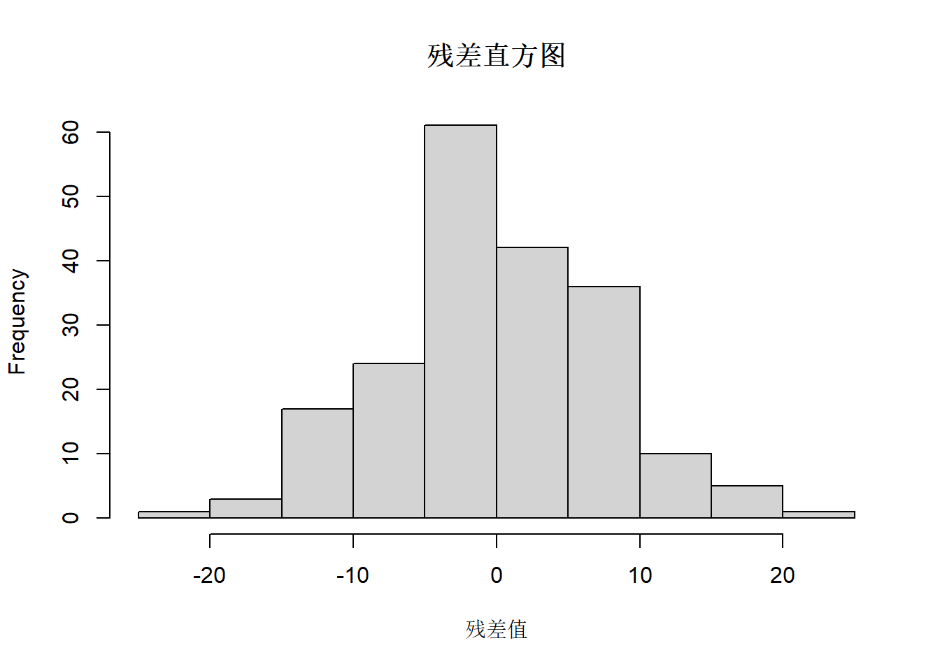
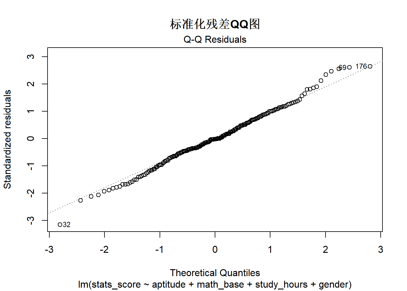
2. 残差正态性检验:绘制残差直方图、标准化残差 QQ 图,QQ 图上的点越贴近对角线,说明残差正态性越好。
hist(resid) \# 残差直方图
plot(fit, which = 2) \# 标准化残差QQ图
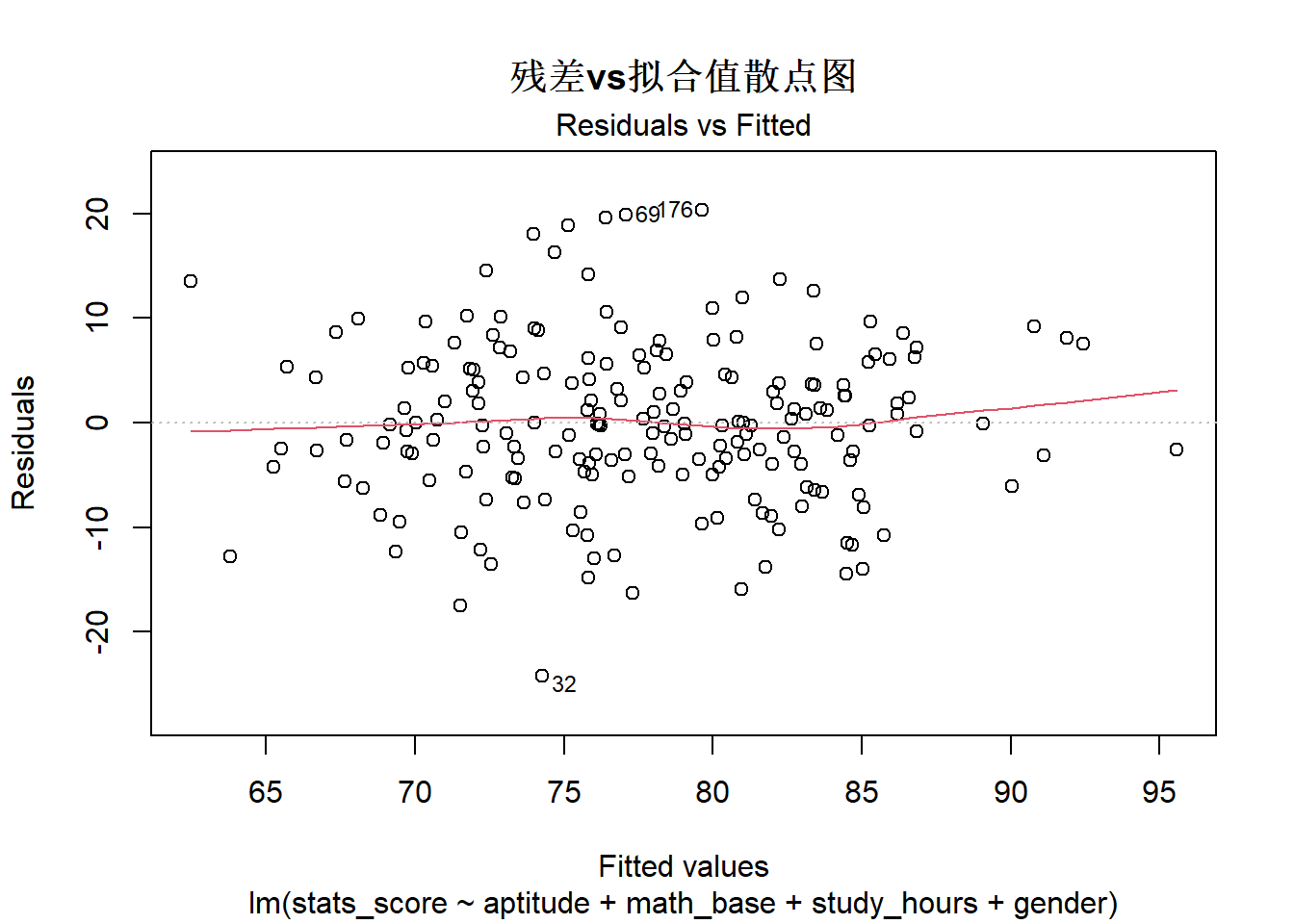
3. 同方差性检验:绘制残差 vs 拟合值的散点图,残差随机分布在 0 线上下、无明显趋势(如漏斗形),说明满足同方差性。
plot(fit, which = 1) \# 残差vs拟合值散点图异常值与强影响点检验\
残差值:绝对值越大,越可能是异常值;\
Cook 距离:\>1 提示为强影响点,会显著改变模型结果;\
杠杆值(Hat 值):超过平均值 2-3 倍为高杠杆点,平均值 =(P+1)\\N;\
马氏距离:衡量样本离自变量均值的距离,过大提示为多元异常值
多重共线性核心公式 $$Tolerance = 1 - R_C^2 \quad \text{VIF} = \frac{1}{\text{Tolerance}}$$
```{r}
#步骤6 模型诊断与前提假设检验
# 加载必备包(car包用于VIF计算,课件标准方法)
# install.packages("car")
#library(car)

# 沿用已拟合的非标准化回归模型(与前序步骤一致)
fit <- lm(stats_score ~ aptitude + math_base + study_hours + gender, data = x_df)

#1. 多重共线性检验
# 计算方差膨胀因子VIF
vif_result <- vif(fit)
# 计算容忍度 Tolerance = 1\VIF
tolerance_result <- 1 / vif_result

# 输出多重共线性结果
cat("多重共线性检验结果\n")
cat("方差膨胀因子VIF:\n"); print(vif_result)
cat("容忍度Tolerance:\n"); print(tolerance_result)
#2. 残差正态性检验
# 提取模型残差
resid <- residuals(fit)
# 残差直方图
hist(resid, main = "残差直方图", xlab = "残差值")
# 标准化残差QQ图(代码:plot(fit, which = 2))
plot(fit, which = 2, main = "标准化残差QQ图")
#3. 同方差性检验
# 残差vs拟合值散点图(代码:plot(fit, which = 1))
plot(fit, which = 1, main = "残差vs拟合值散点图")
# 4. 异常值与强影响点检
# 残差值(绝对值越大越可能异常)
resid_abs <- abs(resid)
# Cook距离(>1为强影响点)
cook_result <- cooks.distance(fit)
# 杠杆值Hat值(平均值=(P+1)\N,超2-3倍为高杠杆)
hat_result <- hatvalues(fit)
hat_mean <- (length(coef(fit)))/nrow(x_df)  # (P+1)\N
# 马氏距离(多元异常值检验)
x_matrix <- model.matrix(fit)[, -1]  # 提取自变量矩阵
mahal_result <- mahalanobis(x_matrix, colMeans(x_matrix), cov(x_matrix))

# 输出异常值核心结果
cat("异常值检验核心指标\n")
cat("杠杆值平均值:", hat_mean, "\n")
cat("Cook距离最大值:", max(cook_result), "\n")
```
### 10.7 模型预测力的收缩估计
交叉验证:将样本拆分为两半,一半拟合模型,一半做预测,计算真实值与预测值的相关系数;
双重交叉验证:交换两半样本重复上述操作,取两个相关系数的平均值;
PRESS 统计量:每次留 1 个样本,用剩下的 N-1 个样本拟合模型预测该样本,重复 N 次,计算残差平方和。\
```{r}
# 模型预测力的收缩估计
# 沿用之前的基准回归模型
fit <- lm(stats_score ~ aptitude + math_base + study_hours + gender, data = x_df)
set.seed(123) # 固定随机数,结果可重复


# 1. 简单交叉验证(样本拆分:一半建模,一半预测)
# 方法:将数据随机分为训练集(50%)、测试集(50%),计算真实值与预测值的相关系数

n <- nrow(x_df)
train_idx <- sample(1:n, size = n/2)  # 随机抽取50%样本作为训练集
train_data <- x_df[train_idx, ]
test_data  <- x_df[-train_idx, ]

# 训练集拟合模型,测试集预测
fit_cv <- lm(stats_score ~ aptitude + math_base + study_hours + gender, data = train_data)
pred_cv <- predict(fit_cv, newdata = test_data)
# 计算真实值与预测值的相关系数
cv_cor <- cor(test_data$stats_score, pred_cv)

# 输出结果
cat("简单交叉验证结果\n")
cat("真实值与预测值的相关系数 =", round(cv_cor, 4), "\n")
# 2. 双重交叉验证(交换样本,取两次相关系数的平均值)
#
# 第一次:训练集1 → 测试集2(已算完:cv_cor)
# 第二次:交换 → 测试集1建模,训练集2预测
fit_cv2 <- lm(stats_score ~ aptitude + math_base + study_hours + gender, data = test_data)
pred_cv2 <- predict(fit_cv2, newdata = train_data)
cv_cor2 <- cor(train_data$stats_score, pred_cv2)
# 双重交叉验证平均值
double_cv_cor <- mean(c(cv_cor, cv_cor2))

cat("双重交叉验证结果\n")
cat("第一次相关系数 =", round(cv_cor, 4), "\n")
cat("第二次相关系数 =", round(cv_cor2, 4), "\n")
cat("双重交叉验证平均相关系数 =", round(double_cv_cor, 4), "\n")
# 3. PRESS 统计量(留一法:每次剔除1个样本,预测该样本,计算残差平方和)

PRESS <- sum((residuals(fit) / (1 - hatvalues(fit)))^2)  # 留一法残差平方和
SSY <- sum((x_df$stats_score - mean(x_df$stats_score))^2) # 总平方和
press_R2 <- 1 - PRESS / SSY  # PRESS 预测R²

cat("PRESS 统计量结果\n")
cat("PRESS 统计量(留一残差平方和) =", round(PRESS, 4), "\n")
cat("PRESS 预测 R² =", round(press_R2, 4), "\n")
```