什么是方差分析?
方差,用来衡量数据的离散程度。
方差分析(Analysis of Variance,ANOVA)用于比较三个或更多组均值是否存在显著差异。它通过分析数据总变异中组间变异与组内变异的比例,判断分组因素对结果的影响是否显著。若组间变异明显大于组内变异,则认为至少有两组均值不同。适用于连续因变
5.1ANCOVA有协变量方差分析
作用:以ANOVA为基础,先剔除连续型协变量对因变量的效应,实现两个核心目标:
减少组内“无法解释的误差方差”,提升检验的统计效力;
消除协变量带来的混杂偏倚,更精准地分析分类自变量对连续因变量的真实效应.
适用范围:原本为单因素\多因素ANOVA问题(因变量连续,自变量为分类变量);
存在连续型协变量:该变量非实验核心操纵变量,但对因变量有显著影响
适用于实验研究\观察性研究(观察性研究可放宽部分假设);
数据满足ANOVA基本假设+ANCOVA特有假设.
H₀:控制协变量后,自变量不同水平下因变量的总体均值相等
(比如说:控制年龄后,不同工作时间组的肺容量总体均值无差异);
协变量假设:协变量对因变量无显著线性效应(即协变量的回归斜率b=0).
算法\计算逻辑:ANCOVA本质是带分类自变量的线性回归模型\[Y_i=b_0+b_1X_1i+b_2⋅Covariate_i\]
举例:
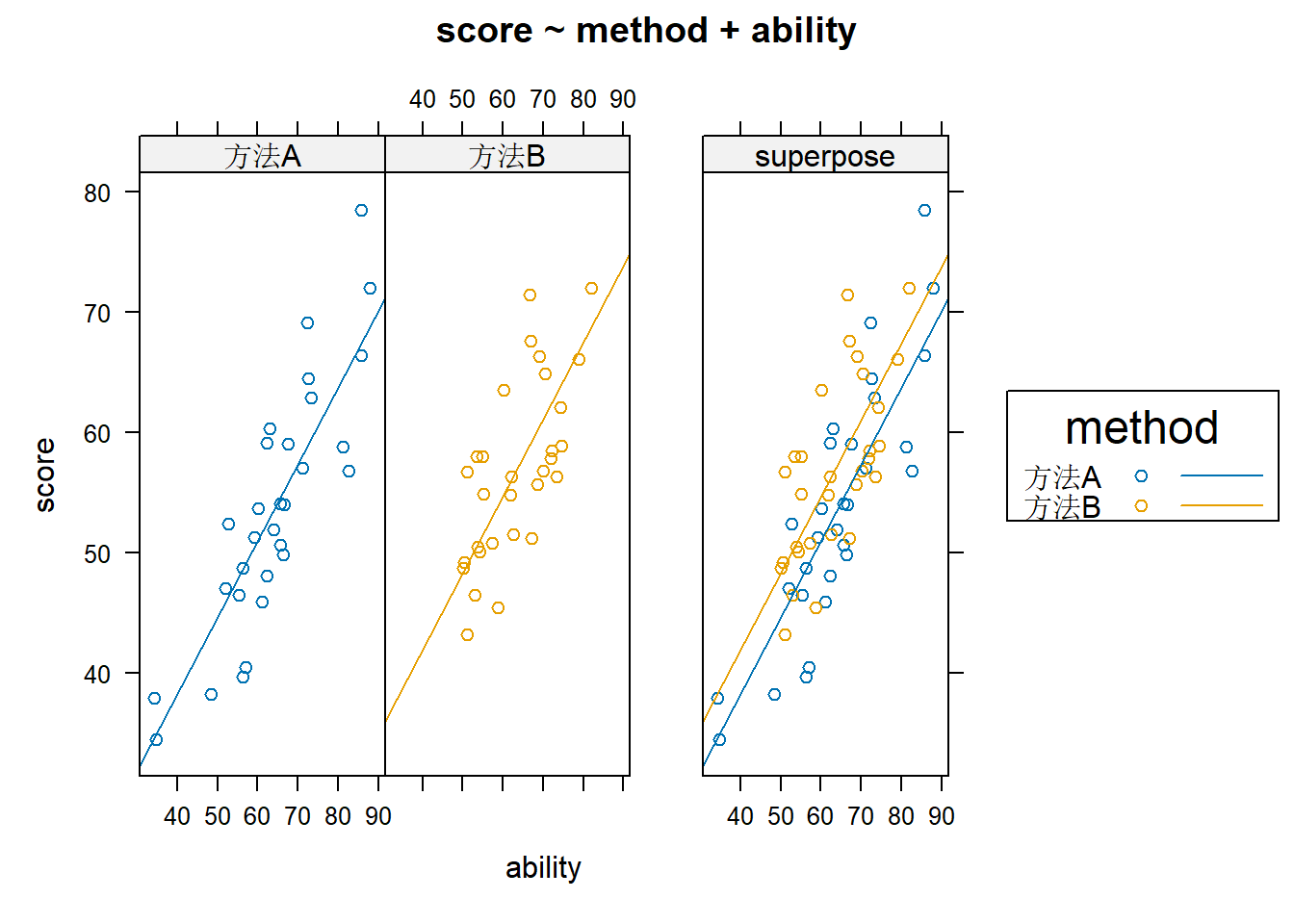
案例背景:研究两种复习方法(自变量:method)对考试分数(因变量:score)的影响, 同时控制学生的基础能力(协变量:ability,连续变量)作为混杂因素。
预期:即便考虑了基础能力差异,复习方法仍对考试分数有显著影响。
数据特点:总体趋势合理,但存在随机误差,不完全理想。
5.1.1 ANCOVA Assumptions前提假设检验
与方差分析相同的假设(方差相等、独立抽样),外加两条:
\[
Y_{i,j} = u + a_j + b \text{ Covariate}_{i,j} + \varepsilon_{i,j}
\] 协变量与处理效应的独立性: 这意味着协变量与X无关
回归斜率同质性(协变量与 X之间无交互作用)
# ANCOVA assumptions ## equal variance ## independence of the covariate and treatment effect ## Homogeneity of regression slopes df <- read_xlsx ( here ( "data" , "excel-files" , "ANCOVA.xlsx" ) ) # 定义变量 y <- df $ score # 因变量:考试分数 x <- as.factor ( df $ method ) # 分组变量:复习方法(方法A / 方法B) covariate <- df $ ability # 协变量:基础能力 # Load the package used to test the assumption of equal variance #library(car) leveneTest ( y ~ x ) # 假设1:方差齐性检验(Levene's Test) # 原理:检验不同分组下因变量的方差是否相等 # leveneTest(因变量 ~ 分组变量, center = median) # center=median:以中位数为中心计算,比均值更稳健 leveneTest ( y ~ x , center = median ) # 若 p > 0.05,接受原假设,满足方差齐性 # 假设2:残差正态性检验(Shapiro-Wilk Test) # 原理:检验模型残差是否服从正态分布(ANCOVA的基础前提) # 先拟合含交互项的回归模型(斜率齐性检验的模型,用其残差做正态性检验) model_interaction <- lm ( y ~ covariate * x ) # 提取残差,做Shapiro-Wilk正态性检验 shapiro.test ( residuals ( model_interaction ) )
    Shapiro-Wilk normality test

data:  residuals(model_interaction)
W = 0.97617, p-value = 0.2884
# 假设3:协变量与处理效应独立性检验 # 原理:检验分组(处理)是否会影响协变量,若分组对协变量无显著影响,则满足独立性 # 方法:单因素ANOVA(协变量 ~ 分组变量) result_independence <- aov ( covariate ~ x ) summary ( result_independence )
            Df Sum Sq Mean Sq F value Pr(>F)
x            1     12   12.33   0.095  0.759
Residuals   58   7532  129.86
# 若 p > 0.05,说明分组对协变量无显著影响,满足独立性假设 # 若 p < 0.05,则协变量与处理相关,ANCOVA 可能不适用 # 假设4:回归斜率齐性检验(核心假设) # 原理:检验协变量与分组的交互项是否显著,不显著则满足斜率齐性 # 方法:含交互项的线性回归\ANOVA(因变量 ~ 分组 * 协变量,* 表示主效应+交互效应) # 原假设:交互项系数为 0,即不同分组中协变量对因变量的回归斜率相同 # 方法:包含协变量、分组及其交互项的 ANOVA / 线性回归 result_slope <- aov ( y ~ x * covariate ) summary ( result_slope )
            Df Sum Sq Mean Sq F value             Pr(>F)
x            1  148.8   148.8   4.903             0.0309 *
covariate    1 3064.0  3064.0 100.941 0.0000000000000386 ***
x:covariate  1   32.5    32.5   1.071             0.3051
Residuals   56 1699.9    30.4
---
Signif. codes:  0 '***' 0.001 '**' 0.01 '*' 0.05 '.' 0.1 ' ' 1
# 注意:输出中 x:covariate 那一行的 p 值
# 若 p > 0.05,则满足斜率齐性假设,可进行标准 ANCOVA
# 若 p < 0.05,说明斜率不同,需考虑其他方法(
5.2 ANCOVA协方差分析
# conduct the test ## Method 1第一种办法 #aov(因变量~自变量+协变量) summary(模型) result = aov ( y ~ x + covariate ) cat ( "\n" )
            Df Sum Sq Mean Sq F value             Pr(>F)
x            1  148.8   148.8   4.897             0.0309 *
covariate    1 3064.0  3064.0 100.815 0.0000000000000324 ***
Residuals   57 1732.4    30.4
---
Signif. codes:  0 '***' 0.001 '**' 0.01 '*' 0.05 '.' 0.1 ' ' 1
# 两种平方和是一样的 Anova ( result , type= "III" )
# Method 2第二种办法 #library('HH') df $ method <- as.factor ( df $ method ) ancova ( score ~ method + ability ,data = df ) #ancova(因变量~自变量+协变量,data=数据来源)
Analysis of Variance Table

Response: score
          Df  Sum Sq Mean Sq  F value             Pr(>F)
method     1  148.84  148.84   4.8972            0.03092 *
ability    1 3064.04 3064.04 100.8150 0.0000000000000324 ***
Residuals 57 1732.38   30.39
---
Signif. codes:  0 '***' 0.001 '**' 0.01 '*' 0.05 '.' 0.1 ' ' 1
# conduct the effect size效应量检验 #library('rstatix') partial_eta_squared ( result )
         x  covariate
0.07911758 0.63881772
5.3 Post-hoc test
# post-hoc test ## Method 1你用了第一种办法就这样时候检验 #library('multcomp')#glht(模型,linfct=mcp(x="Tukey")) postHocs <- glht ( result , linfct = mcp ( x = "Tukey" ) ) summary ( postHocs )
     Simultaneous Tests for General Linear Hypotheses

Multiple Comparisons of Means: Tukey Contrasts


Fit: aov(formula = y ~ x + covariate)

Linear Hypotheses:
                   Estimate Std. Error t value Pr(>|t|)
方法B - 方法A == 0    3.728      1.425   2.617   0.0113 *
---
Signif. codes:  0 '***' 0.001 '**' 0.01 '*' 0.05 '.' 0.1 ' ' 1
(Adjusted p values reported -- single-step method)
## Method 2 #library('emmeans') emmeans ( result , pairwise ~ x , adjust = 'tukey' )
$emmeans
   x   emmean   SE df lower.CL upper.CL
 方法A   53.4 1.01 57     51.3     55.4
 方法B   57.1 1.01 57     55.1     59.1

Confidence level used: 0.95

$contrasts
     contrast  estimate   SE df t.ratio p.value
 方法A - 方法B    -3.73 1.42 57  -2.617  0.0113
#emmeans(模型,pariwise~x,adjust="tukey")
5.4 Ancova & Linear model 模型比较
# the relations between linear model and ANCOVA lresult = lm ( y ~ x + covariate ) summary ( lresult )
Call:
lm(formula = y ~ x + covariate)

Residuals:
   Min     1Q Median     3Q    Max
-8.882 -4.413 -0.615  3.321 12.456

Coefficients:
            Estimate Std. Error t value           Pr(>|t|)
(Intercept) 12.73762    4.19617   3.036            0.00362 **
x方法B       3.72828    1.42460   2.617            0.01134 *
covariate    0.63780    0.06352  10.041 0.0000000000000324 ***
---
Signif. codes:  0 '***' 0.001 '**' 0.01 '*' 0.05 '.' 0.1 ' ' 1

Residual standard error: 5.513 on 57 degrees of freedom
Multiple R-squared:  0.6497,    Adjusted R-squared:  0.6374
F-statistic: 52.86 on 2 and 57 DF,  p-value: 0.000000000000104
# transform the result anova ( lresult ) # model comparison模型比较:检验回归斜率齐性 # Model 1:主效应模型(无交互项)→ 满足斜率齐性假设 m1 <- aov ( y ~ covariate + x , data = df ) # Model 2:交互效应模型(含交互项)→ 检验斜率是否不齐 m2 <- aov ( y ~ covariate * x , data = df ) anova ( m1 , m2 )
6.0 Latin Square拉丁方
作用:针对单因素实验,同时剔除两个相互独立的系统干扰变量(行因素,列因素)的效应,进一步减少误差方差,提升检验力; 消除双维度系统误差的混杂(如田间试验的“行\列位置”,实验的“时间\空间”),更精准分析处理因素(核心自变量)的效应;
让实验设计更高效,避免无关变量对因变量的干扰.
适用范围 仅适用于单因素实验(一个核心处理因素,有p个水平);
存在两个相互独立的干扰变量(行因素,列因素)
\[
\begin{array}{|c|c|c|c|}
\hline &
c_1 & c_2 & c_3 \\
\hline
b_1 & a_1 & a_2 & a_3 \\
\hline
b_2 & a_2 & a_3 & a_1 \\
\hline
b_3 & a_3 & a_1 & a_2 \\
\hline\end{array}
\]
对应的处理组合为: \[
\begin{aligned}& a_1b_1c_1 \quad a_1b_2c_3 \quad a_1b_3c_2 \\& a_2b_1c_2 \quad a_2b_2c_1 \quad a_2b_3c_3 \\& a_3b_1c_3 \quad a_3b_2c_2 \quad a_3b_3c_1\end{aligned}
\]
行因素,列因素,核心处理之间没有关系
设计硬性要求:处理因素的水平数p=行因素水平数=列因素水平数; 拉丁方的排列规则:每个处理在每行,每列仅出现一次(无重复);
处理因素H₀:不同处理水平下因变量的总体均值相等(H0:μ.1..=μ.2..=…=μ.p..,文档中:不同甜菜品种的产量均值无差异);
行因素H₀:不同行的因变量总体均值相等(H0:μ..1.=μ..2.=…=μ..p.,文档中:田间不同行的产量均值无差异);
列因素H₀:不同列的因变量总体均值相等(H0:μ…1=μ…2=…=μ…p.,文档中:田间不同列的产量均值无差异). 算法\计算逻辑 拉丁方的核心是设计+方差分析,模型公式: \[Y_{ijkl}=μ+αj+βk+γl+ϵijkl\] μ:总均值; \(\alpha_j\) :处理因素的效应;\(\beta_k\) :行因素的效应;\(\gamma_l\) :列因素的效应;\(\epsilon_{ijkl}\) :随机误差;
# Latin Square 节省被试量 假设abc不存在交互作用 # 拉丁方设计示例:研究不同肥料对作物产量的影响,控制行(土地肥力梯度)和列(灌溉条件梯度)两个干扰因素 # 假设行、列、处理间无交互作用(拉丁方设计的基本前提) # 处理因素:肥料类型(4 个水平:A、B、C、D) # 行因素:土地肥力区块(4 个水平,从低到高) # 列因素:灌溉条件区块(4 个水平,从差到好) # 每个单元格有 2 个重复观测(共 4×4×2 = 32 个样本) # Load the package used to read .xlsx data #library(readxl) yie = read_xlsx ( here ( "data" ,"excel-files" ,"latin_example.xlsx" ) ) # conduct the test fit = aov ( yield ~ as.factor ( row ) + as.factor ( col ) + as.factor ( treat ) ,data = yie ) summary ( fit )
                 Df Sum Sq Mean Sq F value     Pr(>F)
as.factor(row)    3  400.7  133.57  21.307 0.00000105 ***
as.factor(col)    3   54.8   18.25   2.912     0.0572 .
as.factor(treat)  3  317.8  105.94  16.899 0.00000641 ***
Residuals        22  137.9    6.27
---
Signif. codes:  0 '***' 0.001 '**' 0.01 '*' 0.05 '.' 0.1 ' ' 1
#构建ANOVA模型:因变量~行因素+列因素+处理因素 #fit=aov(yield~as.factor(rep)+as.factor(col)+as.factor(variety),data=yie) #效应检验 Anova ( fit , type = 'III' ) #注意这个函数主要是画图标出来的 # conduct the post-hoc test事后检验 ## Method 1 TukeyHSD ( fit )
  Tukey multiple comparisons of means
    95% family-wise confidence level

Fit: aov(formula = yield ~ as.factor(row) + as.factor(col) + as.factor(treat), data = yie)

$`as.factor(row)`
     diff        lwr      upr     p adj
2-1 2.725 -0.7513103  6.20131 0.1609962
3-1 5.800  2.3236897  9.27631 0.0006922
4-1 9.500  6.0236897 12.97631 0.0000008
3-2 3.075 -0.4013103  6.55131 0.0955659
4-2 6.775  3.2986897 10.25131 0.0001081
4-3 3.700  0.2236897  7.17631 0.0341991

$`as.factor(col)`
      diff         lwr     upr     p adj
2-1 0.6000 -2.87631031 4.07631 0.9628845
3-1 1.8625 -1.61381031 5.33881 0.4613850
4-1 3.4125 -0.06381031 6.88881 0.0555953
3-2 1.2625 -2.21381031 4.73881 0.7461987
4-2 2.8125 -0.66381031 6.28881 0.1419248
4-3 1.5500 -1.92631031 5.02631 0.6101423

$`as.factor(treat)`
       diff      lwr        upr     p adj
B-A  5.8125  2.33619  9.2888103 0.0006758
C-A  1.9375 -1.53881  5.4138103 0.4276433
D-A  8.0250  4.54869 11.5013103 0.0000107
C-B -3.8750 -7.35131 -0.3986897 0.0252115
D-B  2.2125 -1.26381  5.6888103 0.3150023
D-C  6.0875  2.61119  9.5638103 0.0003994
## Method 2 emmeans ( fit , pairwise ~ treat , adjust = 'tukey' )
$emmeans
 treat emmean    SE df lower.CL upper.CL
 A       55.1 0.885 22     53.3     56.9
 B       60.9 0.885 22     59.1     62.7
 C       57.0 0.885 22     55.2     58.9
 D       63.1 0.885 22     61.3     65.0

Results are averaged over the levels of: row, col
Confidence level used: 0.95

$contrasts
 contrast estimate   SE df t.ratio p.value
 A - B       -5.81 1.25 22  -4.643  0.0007
 A - C       -1.94 1.25 22  -1.548  0.4276
 A - D       -8.03 1.25 22  -6.410 <0.0001
 B - C        3.88 1.25 22   3.095  0.0252
 B - D       -2.21 1.25 22  -1.767  0.3150
 C - D       -6.09 1.25 22  -4.863  0.0004

Results are averaged over the levels of: row, col
P value adjustment: tukey method for comparing a family of 4 estimates
7.0Nested ANOVA有嵌套因子的方差分析
作用“:检验主因子的处理效应,同时控制嵌套在主因子内的次级因子的变异;
解决次级因子样本非独立,样本量有限的问题,避免直接用单因素ANOVA导致的假阳性.
适合范围:存在层级\嵌套结构的实验设计,即次级因子(如location\rat\site)嵌套在主因子(如method\technician\habitat)中;
嵌套因子水平随主因子水平变化,无交叉;
可处理平衡\非平衡数据(平衡数据易计算,非平衡需混合模型).
H₀(俩) 主因子效应:\(\alpha_i=0\) ,即主因子各水平下因变量总体均值无显著差异;
嵌套因子效应:\(\beta_{j\left(i\right)}=0\) ,即嵌套因子各水平在对应主因子内无显著差异.
方差来源:
组间(主要因子)df=a-1代表核心因子
组内子组(嵌套因子)df=a(b-1)主要是为防止假阳性
子组内(误差)df=ab(n-1)
总df=abn-1 SS\df=MS,
\[
\begin{array}{|l|c|c|}
\hline
\text{变异来源} & \text{平方和} & \text{自由度} \\
\hline
\text{组间} & SS_{\text{among}} = bn \sum_i (\bar{Y}_{i.} - \bar{Y}_{..})^2 & a-1 \\
\hline
\text{组内子组} & SS_{\text{subgr}} = n \sum_i \sum_j (\bar{Y}_{ij.} - \bar{Y}_{i.})^2 & a(b-1) \\
\hline
\text{子组内} & SS_{\text{within}} = \sum_i \sum_j \sum_k (Y_{ijk} - \bar{Y}_{ij.})^2 & ab(n-1) \\
\hline
\text{总计} & \sum_i \sum_j \sum_k (Y_{ijk} - \bar{Y}_{..})^2 & abn-1 \\
\hline
\end{array}
\]
# nested ANOVA # 嵌套 ANOVA 示例:研究不同教学方法对学生考试成绩的影响 # 教学方法(method)为固定因素,每个方法下随机抽取多个班级(location),班级嵌套在教学法中 # 因变量 DV:考试成绩(百分制) # 结构:method 有两个水平,每个 method 下有 3 个不同的 location(班级),每个班级 10 名学生 # load the data,一定要注意as.factor() #library(here) #library(readxl) nestedData <- read_excel ( here ( "data" , "excel-files" , "nested_anova.xlsx" ) ) nestedData $ method <- as.factor ( nestedData $ method ) nestedData $ location <- as.factor ( nestedData $ location ) # Conduct the correct test ## Method 1 #固定效应,用不着推广的那种 # 注意:Error(location) 表示 location 是嵌套在 method 内的随机因素,但在 aov 中通常用来指定误差分层 cat ( "Method 1: 固定效应嵌套 ANOVA (不推广到总体)\n" )
Method 1: 固定效应嵌套 ANOVA (不推广到总体)
cat ( "模型:DV ~ method + Error(location)\n" )
模型:DV ~ method + Error(location)
aov.result = aov ( DV ~ method + Error ( location ) ,data = nestedData ) summary ( aov.result )
Error: location
          Df Sum Sq Mean Sq F value  Pr(>F)
method     1  992.3   992.3   21.66 0.00963 **
Residuals  4  183.3    45.8
---
Signif. codes:  0 '***' 0.001 '**' 0.01 '*' 0.05 '.' 0.1 ' ' 1

Error: Within
          Df Sum Sq Mean Sq F value Pr(>F)
Residuals 54   1432   26.52
#其实还有别的写法,但是其他的需要手动矫正,为了方便我就不放别的玩意了
## Method 2 #如果地点是随机抽取的,要推广到总体 #混合效应模型:(1|method\location)表示location嵌套在method里的随机效应 cat ( "========================================\n" )
========================================
cat ( "Method 2: 混合效应嵌套 ANOVA (可推广到总体)\n" )
Method 2: 混合效应嵌套 ANOVA (可推广到总体)
cat ( "模型:lmer(DV ~ method + (1 | method/location))\n" )
模型:lmer(DV ~ method + (1 | method/location))
cat ( "========================================\n" )
========================================
#library(lme4) #library(lmerTest) model_lmer <- lmer ( DV ~ method + ( 1 | method / location ) , data = nestedData ) summary ( model_lmer )
Linear mixed model fit by REML. t-tests use Satterthwaite's method [
lmerModLmerTest]
Formula: DV ~ method + (1 | method/location)
   Data: nestedData

REML criterion at convergence: 363.7

Scaled residuals:
     Min       1Q   Median       3Q      Max
-2.92216 -0.61627  0.01874  0.75897  1.72711

Random effects:
 Groups          Name        Variance Std.Dev.
 location:method (Intercept)  1.929   1.389
 method          (Intercept) 99.173   9.959
 Residual                    26.522   5.150
Number of obs: 60, groups:  location:method, 6; method, 2

Fixed effects:
               Estimate Std. Error     df t value      Pr(>|t|)
(Intercept)      67.667     10.035 55.498   6.743 0.00000000956 ***
method创新教学    8.133     14.192 55.498   0.573         0.569
---
Signif. codes:  0 '***' 0.001 '**' 0.01 '*' 0.05 '.' 0.1 ' ' 1

Correlation of Fixed Effects:
8. MANOVA多因素方差分析
示例1
案例背景:研究三种锻炼方案(自变量:exercise)对多项健康指标的影响
因变量:
三种锻炼方案:
8.1 Assumptions(前提假设检验)
观测独立;
无单\多元异常值;
各DV方差齐性(Levene检验)
多元正态性(DV及任意线性组合正态,Shapiro-Wilk\马氏距离检验)
协方差矩阵齐性(Box’sM检验)或者说协方差同质;
DV间不要求线性相关;但因变量无多重共线性(DV间r<0.9,否则结果不稳定).
## Multivariate normality ## Equal variance ## Homogeneity of the covariance matrices ## Linearity # load the data manova_data <- read_xlsx ( here ( "data" , "excel-files" , "MANOVA_example.xlsx" ) ) # 提取因变量矩阵(y1 和 y2) IV <- cbind ( manova_data $ y1 , manova_data $ y2 ) # 自变量:锻炼方案 exercise <- as.factor ( manova_data $ exercise ) cat ( "Assumption 1: Multivariate Normality (多元正态性)\n" )
Assumption 1: Multivariate Normality (多元正态性)
#library('mvnormtest') #library('dplyr') #library('rstatix') # 注意:mshapiro.test 要求输入为矩阵,行是变量,列是样本,故对 IV 转置 mshapiro.test ( t ( IV ) )
    Shapiro-Wilk normality test

data:  Z
W = 0.99003, p-value = 0.7329
# 按分组进行单变量正态性检验(Shapiro-Wilk) manova_data %>% group_by ( exercise ) %>%
shapiro_test ( y1 , y2 ) %>%
arrange ( variable ) cat ( "Assumption 2: Equal Variance (方差齐性)\n" )
Assumption 2: Equal Variance (方差齐性)
leveneTest ( manova_data $ y1 , exercise ) leveneTest ( manova_data $ y2 , exercise ) cat ( "Assumption 3: Homogeneity of Covariance Matrices (协方差矩阵齐性)\n" )
Assumption 3: Homogeneity of Covariance Matrices (协方差矩阵齐性)
#library('heplots') # Box's M 检验:检验各组的协方差矩阵是否相等 boxM ( cbind ( y1 , y2 ) ~ exercise , data = manova_data )
 Box's M-test for Homogeneity of Covariance Matrices

data:  manova_data
Chi-Sq (approx.) = 5.4602, df = 6, p-value = 0.4863
# 线性关系检验:两个因变量之间的相关性(原代码仅作示例) cor.test ( manova_data $ y1 , manova_data $ y2 )
    Pearson's product-moment correlation

data:  manova_data$y1 and manova_data$y2
t = 1.1755, df = 88, p-value = 0.243
alternative hypothesis: true correlation is not equal to 0
95 percent confidence interval:
 -0.08494135  0.32310830
sample estimates:
      cor
0.1243369
8.2 MANOVA Test
# conduct MANOVA cat ( "=============MANOVA整体检验结果===============" )
=============MANOVA整体检验结果===============
          Df  Pillai approx F num Df den Df                Pr(>F)
exercise   2 0.73048    25.03      4    174 < 0.00000000000000022 ***
Residuals 87
---
Signif. codes:  0 '***' 0.001 '**' 0.01 '*' 0.05 '.' 0.1 ' ' 1
cat ( "=============分因变量的单因素ANOVA===============" )
=============分因变量的单因素ANOVA===============
# The ANOVAs for the two DVs separately summary.aov ( fit )
 Response 1 :
            Df  Sum Sq Mean Sq F value        Pr(>F)
exercise     2  984.32  492.16  22.468 0.00000001359 ***
Residuals   87 1905.70   21.90
---
Signif. codes:  0 '***' 0.001 '**' 0.01 '*' 0.05 '.' 0.1 ' ' 1

 Response 2 :
            Df  Sum Sq Mean Sq F value        Pr(>F)
exercise     2  6943.6  3471.8  19.872 0.00000007797 ***
Residuals   87 15200.0   174.7
---
Signif. codes:  0 '***' 0.001 '**' 0.01 '*' 0.05 '.' 0.1 ' ' 1
# effect size效应量 #library(effectsize) effectsize :: eta_squared ( fit )
8.3Post-hoc Test事后检验
# post-hoc # #library packages to conduct the test #library('dplyr') #library('rstatix') # 1. 数据重塑(长格式转换):将 y1 和 y2 合并为一列 # 语法:gather(数据框, key = "变量名列", value = "变量值列", 需转换的列1, 列2, ...) pwc <- manova_data %>% gather ( key = "variables" , value = "value" , y1 , y2 ) %>%
# 2. 按因变量名称分组(分别对 y1 和 y2 做事后检验) group_by ( variables ) %>%
# 3. 执行 Games-Howell 检验(适用于方差不齐且样本量不等的情况) # 语法:games_howell_test(因变量数值 ~ 分组自变量) games_howell_test ( value ~ exercise ) # 4. 输出结果:包含每对组间的差异、置信区间和校正后 p 值 pwc